From FFTs to Quantum Simulations: The Butterfly Connection
Introduction
Today, I want to bring your attention to the butterfly diagram. By the end of this post, I hope to show you that this stunning visualization also gives you almost everything you need to know in order to implement a quantum state simulator and the Fast Fourier Transform (FFT).
For a while I have been working on a quantum state simulator, Spinoza. During the implementation and performance tuning of the simulator, I encountered a memory access pattern that comes up often in the context of Digital Signals Processing (DSP). Namely, the butterfly, data-flow, diagram.

In this video by Reducible, we see the butterfly diagram. Of course, this video is about the FFT so that makes sense.
We’ll now turn to understanding the implementation of quantum state simulators as well as the FFT through the use of this diagram. Just as one would draw out a binary search tree when reasoning about it, the butterfly diagram gives you almost everything you need to derive an implementation of the FFT or a quantum state simulator.
Note I’m no quantum computing or DSP expert. I’m sure there are a lot of things that are hand wavy in this post.
Simulating a Quantum Computer on a Classical machine
Some quantum computing researchers make extensive use of quantum computer simulators. Their code runs quantum algorithms on relatively tiny amounts of qubits, which are simulated using a state vector.
(Footnote) Of course, the simulators themselves are written in a way such that running the same quantum circuits on “real” quantum computers is a matter of a config change.
So let’s look at the quantum state vector.
# [derive(Debug)]
pub struct QuantumStateVector {
  amplitudes: Vec<Complex64>,
}

impl QuantumStateVector {

  pub fn new(num_qubits: usize) -> Self {
    assert!(num_qubits > 0);
    let num_amps = 1 << num_qubits;
    let mut amplitudes = (0..num_amps).map(|_| Complex64::new(0.0, 0.0)).collect();
    amplitudes[0].re = 1.0;
    Self { amplitudes }

  }
}
So what’s all this? Not much. The QuantumStateVector is not much more than a
Vec<Complex64> (or Vec<Complex32>).
As you can see, the number of qubits is used to compute the number of
amplitudes we’ll need to store in the Vec.
Slightly more formally, we can say every quantum state vector of qubits is represented by amplitudes.
If you’re wondering why are amplitudes and complex numbers being used interchangeably, that’s because for our purposes they are exactly the same. Sweet.
Of course, complex numbers are seldom used outside of certain domains. So let’s do a very quick review.
Complex Numbers
What’s a complex number? such that and
From here on out, let’s just stick to the code perspective. So, here’s our amplitude/complex number in code.
# [derive(Debug)]
struct Amplitude {
  real: f64,
  imaginary: f64,
}
It’s basically a 2D point on a plane. In the case of complex numbers, it’s often referred to as the Argand Diagram.
From here on out, we’ll use the
Complex64
type from the num_complex crate for convenience (all the arithmetic
operations for complex nums are already implemented by this crate).
So let’s consider a quantum state composed of qubits. That means we need amplitudes.
That’s all it is. Just an array of 8 complex numbers. The data structure is simple. The computations we apply to it are where things get a bit hairier.
In the quantum world, operations are applied using gates. Specifically, a single-qubit gate is a matrix.
Sweet. But how do we apply a matrix to a quantum state composed of 8 amplitudes? Well you could build up a gigantic matrix (just imagine how big this matrix needs to be if you wanted to do something with 10 qubits). Clearly a quantum computer has much more power (for certain problems) than a classical machine. But it doesn’t have to be this bad from the space complexity perspective.
You may already know that a matrix is usually applied to a vector. This is where the butterfly comes in.
We’re considering the case of qubits. So let’s apply a gate to qubit .
In the case of target qubit 0, We need to take every contiguous pair in our state, put it into the vector, and apply the matrix to it. Specifically, the pairs are:
Target qubit 1?
Target qubit 2?
So let’s put it all together now:
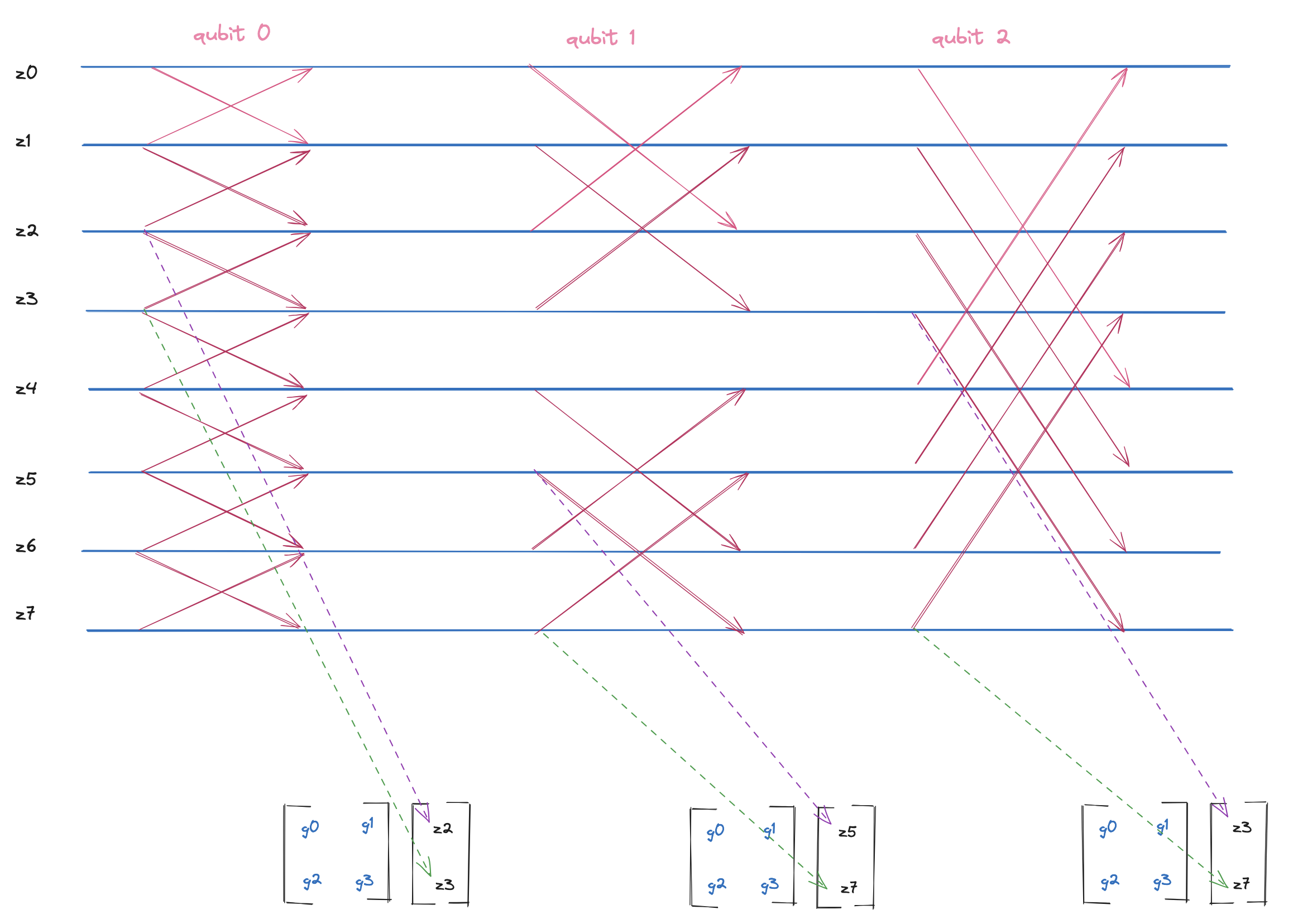
Note how the column labeled qubit 0 shows us retrieving the pair , writing it to the vector. Then we apply the gate (i.e., the matrix) to that vector. The output is another vector whose values need to be overwrite and in the array.
Now let’s see tie this back to quantum computing simulators. We’ll use IBM’s Qiskit SDK to create a super simple quantum circuit that applies the hadamard gate to qubits .
from qiskit import QuantumCircuit

num_qubits = 3
qc = QuantumCircuit(num_qubits)

for qubit in range(num_qubits):
  qc.h(qubit)
Qiskit provides a convenient way to visualize the quantum circuit which we use
to visualize this below. 
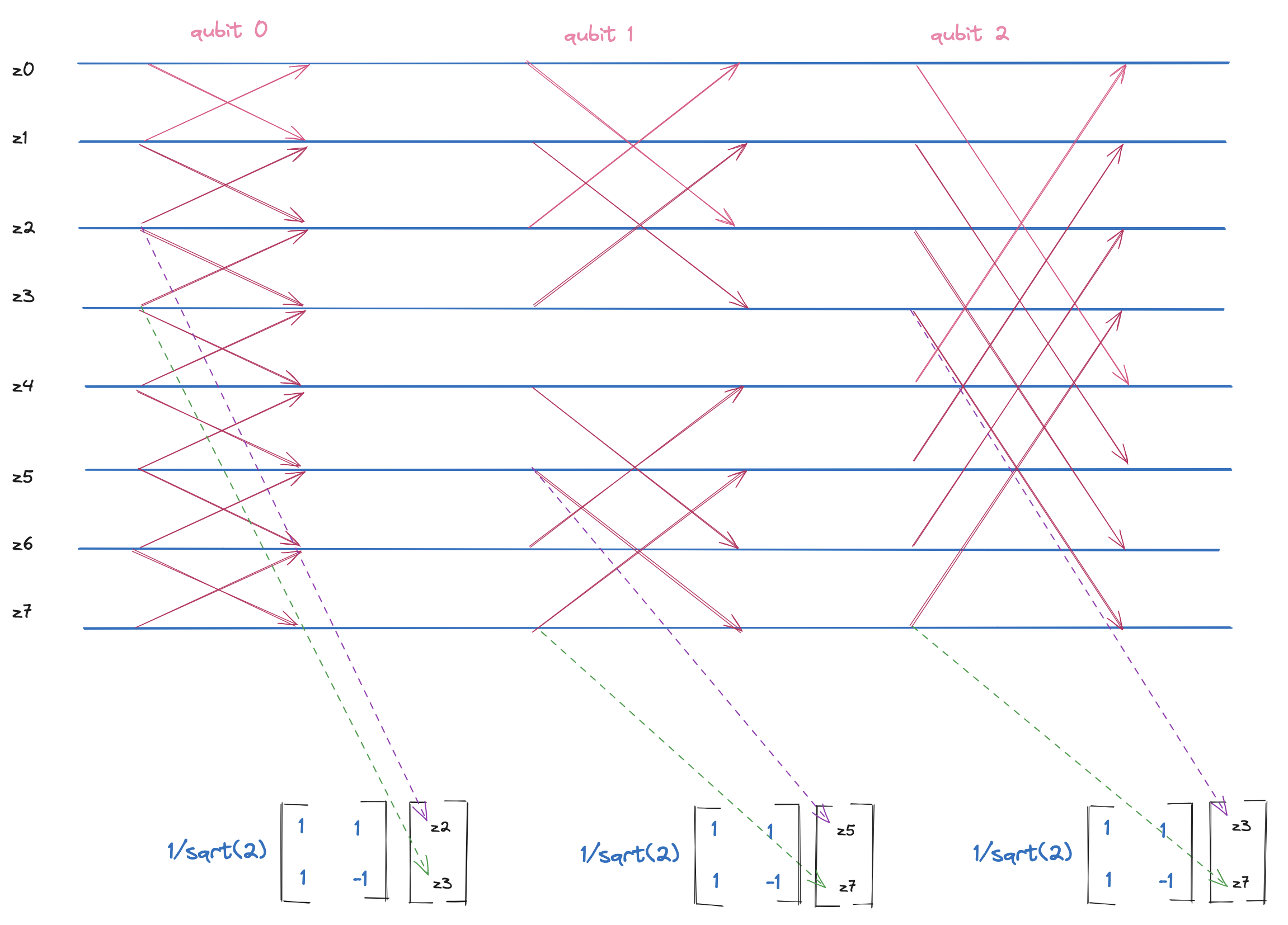
Note how we replace the matrix (i.e., the single-qubit gate) with the actual underlying matrix of the hadamard gate. Now, all corresponding pairs of complex numbers must be multiplied by the hadamard gate. Since our defined circuit applies hadamard to all qubits, we follow the exact data flow as shown in the above diagram.
Finally, let’s look at a slightly larger example where (i.e., a system of 4 qubits), so we have a state composed of amplitudes.
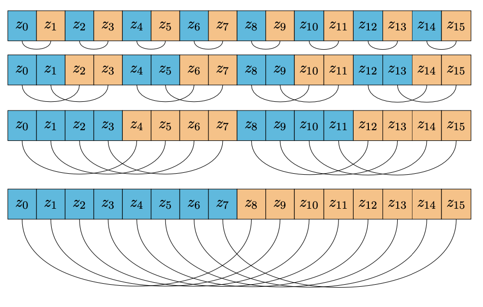
- The 0th row can be thought of as an array composed of chunks.
- The 1st row can be thought of as an array composed of chunks.
- The 2nd row can be thought of as an array composed of chunks.
- The 3rd row can be thought of as an array composed of chunk.
A pattern starts to emerge. Let’s unpack that a bit.
The first row corresponds to the memory access patterns required to apply a single-qubit gate to target qubit . Note how each chunk is composed of amplitudes, and each of those amplitudes corresponds to being on the left/right side of the chunk, or 0 side and 1 side.
The second row corresponds to the memory access patterns required to apply a single-qubit gate to target qubit . Note how each chunk is composed of amplitudes, and the chunk can be bisected at the midpoint to give us two 0-side amplitudes and two 1-side amplitudes.
The third row corresponds to the memory access patterns required to apply a single-qubit gate to target qubit . Note how each chunk is composed of amplitudes, and the chunk can be bisected at the midpoint to give us four 0-side amplitudes and four 1-side amplitudes.
The fourth row corresponds to the memory access patterns required to apply a single-qubit gate to target qubit . Note how each chunk is composed of amplitudes, and the chunk can be bisected at the midpoint to give us eight 0-side amplitudes and eight 1-side amplitudes.
So given a state composed of qubits, we have complex nums. For a given qubit (i.e., 0, 1, 2, 3), we have a stride of , and the size of each chunk at a given stride is .
pub fn apply_gate(state: &mut QuantumState, gate: [[f64; 2]; 2], target_qubit: usize) {
  let stride = 1 << target_qubit; // 2^{t}
  let chunk_size = 2 * stride;  // 2^{t+1}

  let a = Complex64::new(gate[0][0], 0.0);
  let b = Complex64::new(gate[1][0], 0.0);
  let c = Complex64::new(gate[0][1], 0.0);
  let d = Complex64::new(gate[1][1], 0.0);

  for chunk in state.amplitudes.chunks_exact_mut(chunk_size) {
    let (side0, side1) = chunk.split_at_mut(stride);

    for (x, y) in side0.iter_mut().zip(side1.iter_mut()) {
      let u = *x * a + *y * b;
      let w = *x * c + *y * d;
      *x = u; *y = w;
    }
  }
}
This is exactly the code one needs to apply any single qubit gate to a
quantum state vector. Note how simple it is, especially when utilizing Rust’s
std::slice utilities.
Now that we discussed how to utilize the butterfly diagram in order to implement a rudimentary quantum state simulator, let’s turn to the Fast Fourier Transform (FFT).
Deriving the FFT from the Quantum State Simulator
This post is not meant to discuss the theoretical aspects or the background of the FFT. There are a few amazing videos you can watch that cover the FFT. I’d highly recommend the videos by Vertiasium, as well as Reducible. Rather, we want to look at the underlying mechanics of the FFT implementation.
So let’s look at the famous butterfly diagram that always comes up in the context of the FFT.
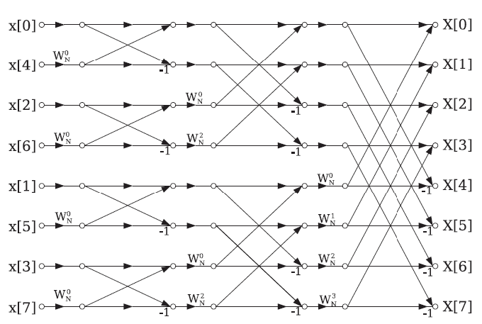 Image source: Optimized
hardware implementation of FFT processor by Al Sallab et al.
Image source: Optimized
hardware implementation of FFT processor by Al Sallab et al.
Does this look familiar? It’s pretty much the same exact diagram as we illustrated above, except we see these factors in the digram, . These are known as twiddle factors.
A twiddle factor, in fast Fourier transform (FFT) algorithms, is any of the trigonometric constant coefficients that are multiplied by the data in the course of the algorithm. This term was apparently coined by Gentleman & Sande in 1966, and has since become widespread in thousands of papers of the FFT literature.
Note how instead of qubits, each vertical column in this diagram is known as a stage. Given a sequence of data of length , there will always be stages in the FFT.
Since we are only considering mechanics and implementation details, just note that rather than using a matrix that’s applied to all pairs, we need to make sure each pair is multiplied by its respective twiddle factor.
Now this section is about to become quite short. Why? Because we already did pretty much 90% of the work to be able to implement the FFT when we implemented our function that applies a single-qubit gate to a quantum state.
pub fn fft_dit(state: &mut QuantumState) {
  let n = state.len().ilog2();

  for stage in 0..n {
    let stride = 1 << stage;        // 2^{t}
    let chunk_size = 2 * stride;    // 2^{t+1}

    for chunk in state.amplitudes.chunks_exact_mut(chunk_size) {
      let (side0, side1) = chunk.split_at_mut(stride);

      for (a, b) in side0.iter_mut().zip(side1.iter_mut()) {
        let a_1 = *a + *b * w;
        let b_1 = *a - *b * w;
        *a = a_1; *b = b_1;
      }
    }
  }
}
The computations in the inner-most loop are even simpler than what we
encountered in the quantum state simulation computations. The only question you
may have at this point is how we can derive that twiddle factor, w to finish
this implementation of the Decimation-in-Time Radix-2 Cooley-Tukey FFT
algorithm.
Discussion
When I first ran into this pattern, I was busy working on implementing a high performance quantum state simulator. An individual on the Rust Discord server ended up telling me that the memory access pattern I illustrated to them was akin to the Decimation-in-Time (DIT) FFT.
After a few months, I ended up looking into the FFT more, and I was astonished to find that the implementations are so similar, anyone that understands the FFT may have an interesting angle to approach and understand quantum computing.
An individual with background in DSP and/or the FFT can have a more intuitive of what quantum computing can do, what it can’t do, and why it has such a significant advantage.
From a performance standpoint, there may be tips and tricks in the implementations of the FFT that can surely be applied in implementations of high-performance quantum state simulators.
Conclusion
Working on Spinoza brought me to the realization that by understanding a rudimentary implementation of a quantum state simulator (i.e., how we access memory to apply gates to respective qubits), we are also able to understand and implement the FFT.
It turns out that a visually stunning diagram that is almost easily reproducible (at least from my unremarkable memory) is all to understand the underlying mechanics of applying gates to qubits and applying the FFT to some sequence of data.
Of course, the butterfly diagram is quite often used in books that cover the FFT; however, there are very few resources that tie that same diagram to quantum computing (or at least simulating a quantum computer on a classical machine).